Oklahoma Candy Onion Production: Projected Net Income, Price Risk, and Yield Risk
Oklahoma producers traditionally produce forages, small grains, and cattle. As national consumption of fruits and vegetables is on the rise1, some producers are selecting alternative enterprises that can help reduce long run income risk. With appropriate planning and market analysis, Oklahoma producers may evaluate their options of producing, promoting, and profiting from alternative enterprises such as onion farming.
A Southeast Oklahoma producer has worked with Dr. Jim Shrefler, Oklahoma State University Extension a Horticulturist; Dr. Merritt Taylor, Director of the Lane Agricultural Center; and USDA-ARS scientists at Lane to evaluate the potential for Oklahoma onion production. Dr. Rodney Holcomb, Oklahoma State University, Food & Agricultural Products Center Food Economist, and Bradley Wathen, Oklahoma State University, Agricultural Economics Extension, have worked in conjunction with the production testing to evaluate specific budgeting and marketing options.
Large-scale onion production does not usually take place in Oklahoma, but according to USDA. data, a large amount of onion production for U.S. markets usually occurs in California, Texas, and Mexico. Three major onion production areas in the United States are Texas, California, and Arizona. Oklahoma’s neighbor to the south poses the most competition for an Oklahoma producer. In the spring of 2003, Texas marketed about 352 million pounds of onions. Can Oklahoma producers be profitable with such a high volume entering the market from the south, and should farmers consider niche markets such as famous Vidalia onions grown in Georgia? A promotional program such as the “Made in Oklahoma” program and finding suitable cultivars, the Candy onion variety for example, may help Oklahoma producers establish their own niche.
Onion production is one of many alternative enterprises for Oklahoma producers. This article will address budgeting and marketing issues so that Oklahoma producers can use the information to make better production decisions should they decide to enter onion production. Awareness of basic onion production and marketing, production budgeting, and marketing risk analyses will help producers advance their knowledge of risks involved with the variables of onion production. Increased knowledge of these few key issues will help producers more properly position themselves, should they decide to enter a market.
Production
Insight into the process of Oklahoma onion production will be useful in further understanding the economic analysis contained herein. Onions are sensitive to temperature and day length. Oklahoma variety trials at the Wes Watkins Research Center/Lane Ag-Center in Lane, Oklahoma2 use short, intermediate, and long day varieties. In trial studies, intermediate day onions do well in Southeast Oklahoma conditions3. The intermediate day Candy onion variety has been, up to this point, the most promising onion for production and marketing purposes in Oklahoma. The Candy variety is, just as the name sounds, a sweet-tasting onion. The sweetness of an onion and other product attributes may be valuable marketing tools for Oklahoma producers.
In an area where predominantly forages, small grains, and cattle are in production, one Oklahoma producer applies conventional row crop and peanut farming machinery to produce onions. In 2003, the producer allotted 10 acres to start an onion production operation for trial purposes. Soil must be tested and then fertilized prior to planting4. Transplanting onions in Oklahoma typically occurs during the second and third week of March.
In Southeast Oklahoma, horticulturists suggest it may not be advantageous to plant on a large scale earlier than March. Weather and soil conditions do not lend themselves to early planting. For this reason, short-day onions, which work well in home gardens, are not acceptable for large-scale plantings and do not reach their production potential. Aside from this, major challenges in Southeast Oklahoma onion production studies include weed control and foliar disease control. Oklahoma State University extension publications are available for helpful information about foliar disease and insect control5.
Water application and timing is important when harvesting in Oklahoma. Production studies prove that when onions do not receive an optimal amount of water, they will not yield to their fullest potential. On the other hand, when onions are watered too much they will sometimes split rendering them useless for fresh markets. Onions, if transplanted in March, should be ready for harvest in June. Once harvest and drying has occurred, onions are graded and packed. Some producers may decide not to grade their onions, which will reduce harvest and marketing costs. The Oklahoma producer referred to earlier in this study does not grade the product and likes to use cardboard boxes that can hold 25 pounds for packaging purposes. Packaging may vary depending on marketing intentions and other variables; however, this study assumes a common 50-pound package size.
In this case the harvested onions are presumably going to market as a fresh product. Therefore, the onions must be in transport as quickly as possible, usually within two weeks of harvest. Transporting onions to market this quickly cuts down on spoilage loss, therefore, helping minimize a decrease in revenue. Marketing the onions as a fresh product is only one option. The producer’s intuition, knowledge of the industry, and willingness to use the mind’s eye are key factors in choosing market and marketing strategy.
Markets and Marketing
Market
“Texas spring onions, which claim 22 percent of the total fresh vegetable value of production in Texas, are by far the largest share of any vegetable crop” (Robinson). Harvesting in late June or July is important because southern region producers with short-day onions will enter the market usually in March through June. “USDA-AMS shipping data between 1990 and 2001 show that an average of 8 percent of the Texas onion crop is marketed during March, 55 percent in April, and the balance is in May and June” (Robinson). “Mexico imports occupy 39 percent and Texas holds 47 percent of U.S. fresh market share in April. In May and early June, 60 percent of the U.S. fresh market is supplied by California, Arizona, and New Mexico, with Texas accounting for 28 percent” (Robinson).
Robinson’s analysis of the Texas onion market resulted in the discovery that a $1 per 50-pound price change in last week’s onion price results in a $0.74 per 50-pound price change in the current week in the same direction, but moderate across multiple weeks of the shipping season. His results indicate that for every 100 truckloads of onions shipped from Mexico and South Texas during the marketing window, onion price declines by $0.108 and $0.105 per 50 pounds, respectively (Robinson). The total number of truckloads going to market in Texas in 2002 consisted of 6,138 in March, 7,857 in April, and 8,903 in May and June. Therefore, if 100 additional truckloads ship during a week in the market window, the producer in this study would experience an $18 decrease in total revenue per acre, using the expected yield in the onion budget (Figure 2).
Marketing
An Oklahoma producer can sell onions through direct or non-direct marketing means6. Concentrating efforts to non-direct marketing activities allows the cooperating producer in this study to sell most or all production at will. Dallas, Texas is the closest and possibly the most feasible regional market for the cooperating Oklahoma producer to market onions. This market is set up like any small town farmer’s market only much larger. Due to possible decreased supply from southern region market suppliers late in the Texas shipping season, Oklahoma onion producers have the possibility of taking and selling all the onions they produce to the Dallas regional market. Having the ability to sell large quantities at once without spending the time that direct marketing efforts require makes non-direct marketing an option worth consideration for producers entering onion production.
Selling in direct markets can restrict a seller in that he/she cannot accurately predict sales volume. Using the direct market option, the producer will usually sell directly to a supermarket or grocery store in the area. The direct option can be beneficial in regards to product price for both the producer and buyer. The farmer is the producer and wholesaler. This affords the farmer an opportunity to receive a higher price at the cost of increased marketing expense for production. Achieving increased final product value is possible if the producer can create a niche market for his/her onion products. Niche markets can be created by generating either real or perceived value for the onion product, i.e. homegrown, super-sweet, Made In Oklahoma, etc. and adding real value by means of processing.
Whether selling through direct or non-direct markets, contracting production can provide further risk management. When contracting, the buyer and seller may wish to set price and/or quantity of product through a legally binding contract with a wholesale broker, supermarket, restaurant, etc. A contract may require a producer to deliver a product that he/she does not have in the event of a crop failure. Therefore, the producer may have to buy product and then resell it to the entity involved in the contract. Under contract, the producer will know he/she has limited sales risk for at least a portion of his/her crop. The risk analysis section of this paper intends to capture the risk aversion affects of contracting production.
Onion Budget
Producers should seek knowledge of what they have to risk in new production practices. The onion budget is a method of seeking this information. After reviewing budgets from Southern California, Florida, and Texas A&M, it was determined that a budget specific to Oklahoma was needed. The cooperation of an Oklahoma producer facilitated the creation of an Oklahoma onion budget. The Oklahoma onion budget will help current and future Oklahoma onion producers analyze their farm’s potential to make a profit. A budget provides the opportunity to estimate expected revenue, expense, and returns to the farm and management over the full growing season before incurring any expense. This onion budget contains two important elements: the operational cost (Figure 1) and summary of revenue and expense (Figures 2, 3, and 4).
Figure 1. Resource use and cost for field operations per arce. (1/3)
| Production Process and Operating Inputs |
Size Per Unit |
Tractor Size hp |
Efficiency Rate hr/acre |
Times Over |
Month |
|---|---|---|---|---|---|
| Chisel Plow | 12' | 135 | 0.11 | 1.0 | 9.0 |
| Heavy Disk | 14' | 135 | 0.10 | 1.0 | 9.0 |
| Heavy Disk | 14' | 135 | 0.10 | 1.0 | 9.0 |
| Disk Bed (Hipper) | 6R-40 | 190 | 0.11 | 1.0 | 1.0 |
| Fert App. | 6R-40 | 55 | 0.19 | 1.0 | 3.0 |
| fert 9-23-30 | Cwt | 3.0 | |||
| Transplanter | 6R-40 | 55 | 1.50 | 1.0 | 3.0 |
| Plants | Unit | ||||
| Spray(18 Row) | 27' | 80 | 0.08 | 1.0 | 3.0 |
| Prowl | Pt | ||||
| Ditcher | standard | 135 | 0.02 | 1.0 | 3.0 |
| Labor (Irr. Setup) | hour | ||||
| Labor (Flood) | hour | 1.0 | 3.0 | ||
| Irr. Water | ac-ft | ||||
| Early Cultivation | 3R-80 | 135 | 0.08 | 1.0 | 4.0 |
| Fert App. | 6R-40 | 55 | 0.19 | 1.0 | 4.0 |
| fert 46-0-0 | Cwt | 4.0 | |||
| Spray(18 Row) | 27' | 80 | 0.08 | 2.0 | 4.0 |
| Prowl | Pt | ||||
| Goal (2XL) | Qt | ||||
| Ditcher | standard | 135 | 0.02 | 1.0 | 4.0 |
| Labor (Irr. Setup) | hour | ||||
| Labor (Flood) | hour | 1.0 | 11.0 | ||
| Irr. Water | ac-ft | ||||
| Spray(18 Row) | 27' | 80 | 0.08 | 1.0 | 11.0 |
| Labor (Flood) | hour | 1.0 | 4.0 | ||
| Irr. Water | ac-ft | ||||
| Spray(18 Row) | 27' | 80 | 0.08 | 1.0 | 5.0 |
| Goal (2XL) | Qt | ||||
| Spray(18 Row) | 27' | 80 | 0.08 | 2.0 | 5.0 |
| Ammo | Lb | ||||
| Bravo Ultrex | Qt | ||||
| Cult and Post (Late) | 6R-40 | 135 | 0.08 | 1.0 | 5.0 |
| Ditcher | standard | 135 | 0.02 | 1.0 | 5.0 |
| Labor (Irr. Setup) | hour | ||||
| Labor (Flood) | hour | 1.0 | 5.0 | ||
| Irr. Water | ac-ft | ||||
| Harvest Onions | Box | 1.0 | 6.0 | ||
| Drying Onions | Box | 1.0 | 6.0 | ||
| Boxes | Box | 1.0 | 6.0 | ||
| Pack and Count Onions | hr/box | 1.0 | 6.0 | ||
| Delivery | miles | 1.0 | 6.0 | ||
Figure 1. Resource use and cost for field operations per arce. (CONTINUED 2/3)
| Production Process and Operating Inputs |
Size Per Unit |
Tractor Cost Variable Dollars |
Tractor Cost Fixed Dollars |
Equipment Cost Variable Dollars |
Equipment Cost Fixed Dollars |
|---|---|---|---|---|---|
| Chisel Plow | 12' | 1.2 | 1.6 | 1.4 | 3.4 |
| Heavy Disk | 14' | 1.0 | 1.3 | 1.3 | 2.2 |
| Heavy Disk | 14' | 1.0 | 1.3 | 1.3 | 2.2 |
| Disk Bed (Hipper) | 6R-40 | 1.7 | 2.0 | 2.7 | 3.4 |
| Fert App. | 6R-40 | 0.8 | 1.4 | 0.5 | 0.6 |
| fert 9-23-30 | Cwt | ||||
| Transplanter | 6R-40 | 6.3 | 11.3 | 11.1 | 9.5 |
| Plants | Unit | ||||
| Spray(18 Row) | 27' | 0.6 | 0.8 | 0.9 | 1.2 |
| Prowl | Pt | ||||
| Ditcher | standard | 0.2 | 0.3 | 0.2 | 0.2 |
| Labor (Irr. Setup) | hour | ||||
| Labor (Flood) | hour | ||||
| Irr. Water | ac-ft | ||||
| Early Cultivation | 3R-80 | 1.1 | 1.1 | 0.9 | 1.6 |
| Fert App. | 6R-40 | 0.5 | 1.4 | 0.5 | 0.6 |
| fert 46-0-0 | Cwt | ||||
| Spray(18 Row) | 27' | 1.2 | 1.7 | 1.8 | 2.4 |
| Prowl | Pt | ||||
| Goal (2XL) | Qt | ||||
| Ditcher | standard | 0.2 | 4.0 | 0.2 | 0.2 |
| Labor (Irr. Setup) | hour | ||||
| Labor (Flood) | hour | ||||
| Irr. Water | ac-ft | ||||
| Spray(18 Row) | 27' | 0.6 | 0.8 | 0.9 | 1.2 |
| Labor (Flood) | hour | ||||
| Irr. Water | ac-ft | ||||
| Spray(18 Row) | 27' | 0.6 | 0.8 | 0.9 | 1.2 |
| Goal (2XL) | Qt | ||||
| Spray(18 Row) | 27' | 1.2 | 1.7 | 1.8 | 2.4 |
| Ammo | Lb | ||||
| Bravo Ultrex | Qt | ||||
| Cult and Post (Late) | 6R-40 | 1.1 | 1.1 | 0.9 | 1.6 |
| Ditcher | standard | 0.2 | 0.3 | 0.2 | 0.2 |
| Labor (Irr. Setup) | hour | ||||
| Labor (Flood) | hour | ||||
| Irr. Water | ac-ft | ||||
| Harvest Onions | Box | ||||
| Drying Onions | Box | ||||
| Boxes | Box | ||||
| Pack and Count Onions | hr/box | ||||
| Delivery | miles | ||||
| Totals | 19.2 | 33.1 | 27.3 | 34.1 | |
Figure 1. Resource use and cost for field operations per arce. (CONTINUED 3/3)
| Production Process and Operating Inputs |
Size Per Unit |
Allocated Labor Hours |
Allocated Labor Cost Dollars |
Operating Input Amount |
Operating Input Price Dollars |
Operating Input Cost Dollars |
Total Cost US Dollars |
|---|---|---|---|---|---|---|---|
| Chisel Plow | 12' | 0.1 | 0.8 | s | $8.40 | ||
| Heavy Disk | 14' | 0.1 | 0.7 | $6.50 | |||
| Heavy Disk | 14' | 0.1 | 0.7 | $6.50 | |||
| Disk Bed (Hipper) | 6R-40 | 0.1 | 0.8 | $10.50 | |||
| Fert App. | 6R-40 | 0.2 | 1.3 | $4.70 | |||
| fert 9-23-30 | Cwt | 4.0 | 15.0 | 60.0 | $60.00 | ||
| Transplanter | 6R-40 | 1.5 | 10.5 | $48.60 | |||
| Plants | Unit | 2.0 | 100.0 | 200.0 | $200.00 | ||
| Spray(18 Row) | 27' | 0.1 | 0.6 | $4.10 | |||
| Prowl | Pt | 0.5 | 2.8 | 1.4 | $1.40 | ||
| Ditcher | standard | 0.0 | 0.1 | $1.00 | |||
| Labor (Irr. Setup) | hour | 0.1 | 0.7 | 0.1 | $0.70 | ||
| Labor (Flood) | hour | 1.0 | 7.0 | 1.0 | $7.00 | ||
| Irr. Water | ac-ft | 0.5 | 10.0 | 5.0 | $5.00 | ||
| Early Cultivation | 3R-80 | 0.1 | 0.6 | $5.30 | |||
| Fert App. | 6R-40 | 0.2 | 1.3 | $4.40 | |||
| fert 46-0-0 | Cwt | 2.0 | 15.0 | 29.9 | $29.90 | ||
| Spray(18 Row) | 27' | 0.1 | 0.6 | $7.60 | |||
| Prowl | Pt | 0.5 | 2.8 | 1.4 | $1.40 | ||
| Goal (2XL) | Qt | 0.5 | 28.0 | 14.0 | $14.00 | ||
| Ditcher | standard | 0.0 | 0.1 | $4.60 | |||
| Labor (Irr. Setup) | hour | 0.1 | 0.7 | 0.1 | $0.70 | ||
| Labor (Flood) | hour | 1.0 | 7.0 | 1.0 | $7.00 | ||
| Irr. Water | ac-ft | 0.4 | 10.0 | 4.0 | $4.00 | ||
| Spray(18 Row) | 27' | 0.1 | 0.6 | $4.10 | |||
| Labor (Flood) | hour | 1.0 | 7.0 | 1.0 | $7.00 | ||
| Irr. Water | ac-ft | 0.5 | 10.0 | 5.0 | $5.00 | ||
| Spray(18 Row) | 27' | 0.1 | 0.6 | $4.10 | |||
| Goal (2XL) | Qt | 0.5 | 28.0 | 14.0 | $14.00 | ||
| Spray(18 Row) | 27' | 0.1 | 0.6 | $7.60 | |||
| Ammo | Lb | 1.0 | 12.0 | 12.0 | $12.00 | ||
| Bravo Ultrex | Qt | 1.0 | 33.0 | 33.0 | $33.00 | ||
| Cult and Post (Late) | 6R-40 | 0.1 | 0.6 | $5.30 | |||
| Ditcher | standard | 0.0 | 0.1 | $1.00 | |||
| Labor (Irr. Setup) | hour | 0.1 | 0.7 | 0.1 | $0.70 | ||
| Labor (Flood) | hour | 1.0 | 7.0 | 1.0 | $7.00 | ||
| Irr. Water | ac-ft | 0.5 | 10.0 | 5.0 | $5.00 | ||
| Harvest Onions | Box | 144.6 | 0.8 | 108.4 | $108.40 | ||
| Drying Onions | Box | 144.6 | 0.2 | 28.9 | $28.90 | ||
| Boxes | Box | 144.6 | 1.2 | 173.5 | $173.50 | ||
| Pack and Count Onions | hr/box | 0.2 | 144.6 | 7.0 | 202.4 | $202.40 | |
| Delivery | miles | 397.5 | 0.4 | 159.0 | $159.00 | ||
| Totals | 7.4 | 50.5 | 1,056 | $1,220.90 | |||
Figure 2: Excel, Summary spreadsheet
| Yield projection | 7,228 | |
|---|---|---|
| Expected Yield | 8,285 | |
| Pounds per box | 50 | |
| Boxes per/acre | 144.56 | |
| Contract Rate | 50.00% |
Figure 3: Excel Onion Production Workbook, Summary spreadsheet, Revenue projections
| Item Revenue | Unit | Price USD | Quantity | Total USD |
|---|---|---|---|---|
| Candy Sweet Yellow Onion | 50 lb. Box | 12.23 | 72.28 | 883.98 |
| Contracted Candy Sweet | 50 lb. box | 22.00 | 72.28 | 1,590.16 |
| Total Revenue | 2,474.14 |
Figure 4: Excel Onion Production Workbook, Summary spreadsheet, Costs projection8
| Item Direct Expense | Unit | Price USD | Quantity | Total USD |
|---|---|---|---|---|
| Fertilizer | ||||
| Fertilizer 9-23-30 | Cwt | 15.00 | 4.00 | 60.00 |
| Fertilizer 46-0-0 | Cwt | 14.95 | 2.00 | 29.90 |
| Fungicide | ||||
| Bravo Ultrex | Qt | 32.95 | 1.00 | 32.95 |
| Herbicide | ||||
| Prowl | Pt | 2.75 | 1.00 | 2.75 |
| Goal 2XL | Qt | 28.00 | 1.00 | 28.00 |
| Insecticide/Miticide | ||||
| Ammo | Lb | 11.95 | 1.00 | 11.95 |
| Irrigation Supplies | ||||
| Water | Ac-ft | 10.00 | 1.50 | 15.00 |
| Seed/Plants | ||||
| Plants | Unit | 100.00 | 2.00 | 200.00 |
| Harvest and Marketing | ||||
| Harvest Onions | 50 lb. Box | 0.75 | 145 | 108.42 |
| Drying Onions | 50 lb. Box | 0.20 | 145 | 28.91 |
| Boxes | 50 lb. Box | 1.20 | 145 | 173.47 |
| Pack Onions | hours per box | 7.00 | 0.20 | 202.38 |
| Delivery | Mile | 0.40 | 397.54 | 159.02 |
| Operator Labor | ||||
| Tractor | Hour | 7.00 | ||
| Hand Labor | ||||
| Implements | Hour | 7.00 | ||
| Irrigation Labor | ||||
| Irrigation setup | Hour | 7.00 | ||
| Labor Flood | Hour | 7.00 | ||
| Unallocated Labor | Hour | 7.00 | 0.15 | 1.05 |
| Interest on capital | Acre | 77.75 | 1 | 77.75 |
| Total Direct Expense | (1,232.57) | |||
| Returns Above Direct Expenses | 1,241.57 | |||
| Fixed Expenses | ||||
| Equipment | 34.07 | 1.00 | 34.07 | |
| Tractors | 33.06 | 1.00 | 33.06 | |
| Total Fixed Expense | (67.13) | |||
| Total Direct and Fixed Expense | (1,299.70) | |||
| Returns Above Total Direct and Fixed Expense | 1,174.44 | |||
| Allocated Cost Items | ||||
| Cash Rent and/or Foregone Income | 100.00 | 1.00 | (100) | |
| Total Expense | (1,399.70) | |||
| Net Income | 1,074.44 | |||
8 The budget was derived with the help and guidance of Dr. Taylor, Dr. Holcomb, Oklahoma State University scientists, a Southeast Oklahoma producer, and examples from Texas A & M.
Figure 5: Long run mean (average) per acre income projections 9
| Contract Rate | Contract Price $22.00/50lbs |
Contract Price $12.50/50lbs |
Contract Price $10.35/50lbs |
Contract Price $8.00/50lbs |
|---|---|---|---|---|
| Contract Rate 0% | $192 | $192 | $192 | $192 |
| Contract Rate 50% | $1.13 | $366 | $193 | $3 |
| Contract Rate 100% | $2,076 | $541 | $193 | ($186) |
| Absolute Minimum Income | Absolute Maximum Income | |||
| Contract Rate 0% Contract Price $8-$22 |
($1,421) | $2,070 | ||
| Contract Rate 50% Contract Price $8-$22 |
($833) | $2,229 | ||
| Contract Rate 100% Contract Price $8-$22 |
($255) | $2.43 | ||
9 Absolute minimum and maximum income is only relevant for the price range of $8.00 to $22.00 per 50lbs.
Operational Cost
The operational cost worksheet (Figure 1) in the budget has many aspects. All costs are on a per acre basis.
- Machinery Cost Formulations
- Formulas that calculate the cost of using a tractor and its equipment per hour that will then be converted to a cost per acre
- Production process and operating inputs
- Machinery and other production inputs
- Size per unit and tractor size
- Unit measure
- Efficiency Rate
- Efficiency rate of a tractor and equipment, hr/acre
- Times over
- Number of times a particular application is applied over a complete acre
- Month
- The month that the application is applied
- Tractor and Equipment Cost
- Variable and Fixed
- Variable cost is a level of specific current production cost that varies with the level of output or input.
- Fixed cost is a specific form of production cost that does not vary with the level of output or input.
- Cost per hour from the machinery cost formulations are adjusted to a per acre cost when multiplied by the hours per acre coefficient.
- Variable and Fixed
- Operating Input Cost
- Amount of operating input (i.e. fertilizer) multiplied by the price of that input equals the cost of that operating input.
- Total Cost
- Summation of all cost within a row for any given input.
- Total Specified Cost
- Summation of the column of total costs.
The operational cost worksheet contains two main components: the machinery cost formulations and the cost estimations for the production process.
Machinery cost is the cost that occurs on the farm when using farm machinery. The machinery cost formulations closely represent the actual cost incurred during the production process on the 10-acre onion test plot of the cooperating Oklahoma producer. The cost of the production process includes the machinery cost and other direct inputs such as labor, fertilizer, and water. Harvest and marketing cost are dependent on yield, which include harvesting and drying of the onions and purchasing boxes, packing, and delivery of the onions, respectively.
Notable assumptions for the onion budget are:
- Continuity
- The production budget assumes that all production resources and activities are continuous.
- Homogeneity
- All units of resources and output are assumed identical.
- Each machine is depreciated over 10 years
- Depreciation per year =
(purchase price-investment credit-salvage value) / (Years of expected life for the machine) x 0.85
- Depreciation per year =
- Input prices are fixed.
- List price of the machinery is assumed to be an average of major national distributors.
- Machinery housing cost is assumed to be 68 cents per square foot per year needed.
- Housing per year = priceper square foot x square feet shelter required
- All units are assumed to be diesel powered.
- Lubrication cost are 5 percent of fuel cost.
- Interest on operating capital was not included in the formulas so that each owner/operator may adjust this value for his/her own application.
- Production is assumed to be sold at a fresh market for human consumption or, another option, as animal feed.
- All production is assumed to be first sold on a fresh vegetable market where the onions
will be most valuable, then sold to other enterprises.
- Other enterprises may use onions as an animal feed. A 1-pound onion will provide 170 kcal of energy and 3.6 grams of protein.
- Onions contain n-propyl disulfide and will cause hemolysis (red blood cell destruction) when fed in excess. Cattle are the most susceptible species to onion toxicity. Onions are toxic to some animals at a ratio of 1 ounce per 3.42 kilograms or less of body weight. A 120-pound animal could be intoxicated by a 1-pound onion.
- In certain rare cases, a producer may choose to pay someone to remove product (spoilage) from his/her possession. In this case, a producer would incur a negative price for production.
- The Simetar simulations do not account for a negative price. The actual Simetar simulation distribution has a mean of $10.34, standard deviation of $3.51, and minimum and maximum of $0.29 and $21.13, respectively.
Summary of Revenue and Expense
The three out-of-state budgets used conventional onion production practices. Conventional onion production practice requires less land use but more human capital than practices used in this analysis. The national average yield is about 40,000 pounds of onions per acre. Potential Oklahoma production of 15,000 to 18,000 pounds per acre is possible with the correct variety and the same production method as used by the cooperating farmer7. Oklahoma State University scientists indicate that the cooperating producer’s plant spacing within each row of onions is larger than needed. In 2003, the cooperating producer’s yield was 8,285 pounds per acre. Manipulating the expected yield of 8,285 pounds per acre in the onion budget (Summary Sheet, Figure 2) returns a representation of yield as dependent on historic values.
Yield has a significant affect on revenue. Revenue is the total dollar amount of sales in a specific period subtracted from total costs. The onion production budget assumes two ways of creating revenue: non-direct sales and non-direct sales by way of contract agreements. A producer will experience price risk when less than 100 percent of the onions sold do not have a predetermined price. An example of budget revenue per acre appears in Figure 3.
Yield not only affects revenue, but also harvest expense. When yield is higher than expected, variable expense is increased and vice versa (Figure 4, Harvest and Marketing). A per acre yield increase will increase labor time used for harvest, drying, and packing the onions. It should be obvious that additional/fewer box purchases will fluctuate with yield; however, it may not be so evident that delivery cost will increase as well. Delivery cost may increase as yield increases depending on transport methods devoted to onions.
The expense/income summary (Figure 4) provides a quick glance at input use and total cost of direct inputs related to onion production. All costs and revenues are on a per acre basis and do not include any returns to operator management. Cost and revenue can change with scale or size of operation. When reviewing the numbers in the example budget (Figures 1-4), keep in mind that this budget uses a program called Simetar, and the output in the “examples” may not represent a likely outcome. Simetar uses distributions based on historical data or other inferences to adjust specified values and analyze risk. Therefore, the static nature of the budget in this manuscript (Figure 1-4) is not as robust as it is when we do an actual Simetar analysis (Figures 6-9).
Figure 6
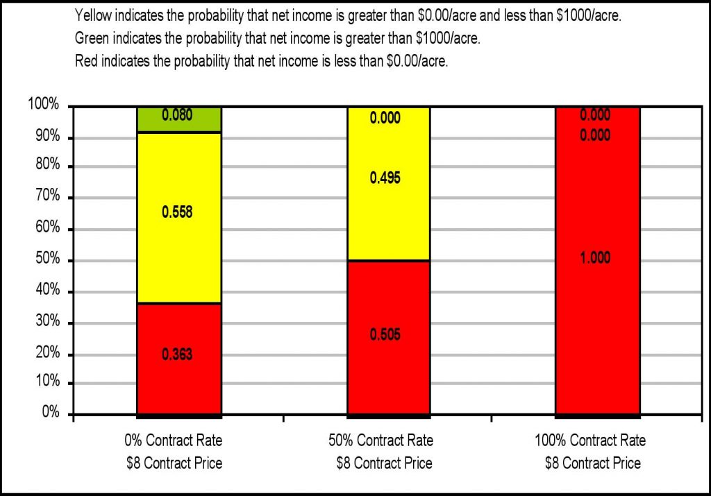
Figure 7

Figure 8.

Figure 9: Contract rate and contract price associated with the zero risk of less than zero net income.
| Contract Rate | Contract price needed to produce a net income of at least $0.00 or greater | |
|---|---|---|
| 25% | $34.05 | |
| 50% | $17.25 | |
| 75% | $12.25 | |
| 100% | $9.82 |
Risk Analysis
In financial terms, risk is a chance that returns on an actual investment is not what is expected. In these analyses, the foundation of risk is related to the uncertainty of input prices from day to day, output prices from day to day, and yield from season to season. On a day-to-day basis, producers in Oklahoma are faced with business decisions that will affect their return in the long run.
“The fact that farmers have to make decisions simply implies that they are faced with alternatives. The alternative actions could be different combinations of crops to produce, alternative production systems for crops or livestock, or different marketing or financial strategies for an agribusiness. If the decisions are to be made in a risk free setting, the manager can easily determine the best strategy… the one with the greatest economic return. When decisions are to be made in a risky environment, the manager cannot use such a simple rule because the economic return for each alternative is a distribution of returns rather than a single value” (James W. Richardson, Creator of Simetar).
Dr. Richardson helped in developing a program to measure risk called Simetar. With Simetar, instead of using fixed variables that give a deterministic outcometo a model, variables that have a known distribution and make a model stochastic are preferred. Making a model stochastic will allow the output of the model to be much more robust when compared to a deterministic model. The variables used to make this model stochastic are:
- Yield
- Remember in the model that yield differences will directly affect the budget cost of inputs and quantity of output.
- Price of output
In this case, these variables have either a historical or a perceived distribution thus allowing the entry of that distribution for the respective variable into the onion production budget. Historical data is preferred; however, there is not enough historical data for production of Oklahoma onions. Since historical data was not available to make a normal distribution of onion production in Oklahoma, it was necessary to seek out a distribution that will appropriately represent probable outcomes without a large number of data points.
The GRK distribution, if just a few years of data are available, could be used. The Simetar GRK distribution was developed by Gray, Richardson, andKlose (Richardson, Simetar). This distribution was developed for subjective probability distributions with little input data. A user can input into Simetar three data points: minimum, median, and maximum. A few properties of the GRK distribution are:
- 50 percent of the simulated observations are less than mid point.
- 95 percent of the simulated observations are between minimum and maximum.
- 2.2 percent of the simulated observation are less than the minimum.
The GRK may be a more appropriate distribution than a uniform distribution for yield data, however without enough data using the seemingly more appropriate distribution is not justified. It may be obvious that the minimum would be zero, but how do we choose a median and maximum data point? For this reason, a more simple distribution was chosen – a uniform distribution.
A uniform distribution allows all simulations to have an equal chance at choosing any data point within a predetermined minimum and maximum. It was assumed that yield will most likely vary by 10 to 15 percent from the current year’s yield. However, in the long run, production practices will change and the Oklahoma producer will begin to plant the variety that creates the most return for his/her business and each variety may have yield variations. The chosen expected yield was 8,285 pounds per acre based on one producer’s 2003 yield. For now, the higher bound of the yield distribution is 10 percent more than 8,285 and the lower bound for yield is 15 percent less than 8,285. This sets the minimum and maximum bounds at 7,042.25 and 9,113.50 pounds of onion production per acre, respectively.
Texas and Mexico medium yellow onion price data for the years of 1999-2003 were gathered. The onion mean price of $10.34 has a variance of 12.42. The onion price has a minimum and maximum of $6.75 and $22.00 per 50 pounds, respectively. A mean price indicates that, on average, medium yellow onion prices were close to $10.34 per 50 pounds, and the variance indicates that, in this case, prices vary by a large amount. Large variance creates more risk for a producer wanting to sell in the open market. Knowing this information helped in determining that a normal distribution should be used for onion price. The normal distribution for the onion budget was set with a mean of $10.34 and a standard deviation of $3.52.
After having found the appropriate distributions for the random variables, simulation could begin. An iteration test indicates that 400 iterations should be used when conducting these Simetar analyses. The objective of simulating 400 iterations is to determine the risk involved with open market sales versus contracting sales during 400 seasons.
Initially, contract rates and contract prices are set. There were three different contract rates used for each of the four different contract prices, thus 12 scenarios in all. Several inferences are possible when reviewing the output of the mean net incomes per acre analysis.
The mean income projections table indicates that contracting at any price below the indifference price of $10.35 per 50 pounds will generate, in the long run, less income than if selling in the open market. The indifference price is $10.35 per 50 pounds because at different contract rates, mean incomes all converge at the price of $10.35. A producer may have long run income incentive to participate in the open market if he/she cannot set a contract price above $10.35. Conversely, there is some income incentive to contract production at any price above $10.35. That is, long run income or residual return increases as the contract price is any price larger than $10.35 per 50 pounds as shown with the contract price of $12.50 per 50 pounds and $22.00 per 50 pounds. These results have illustrated how valuable contracting can be to reduce risk, but bear in mind that income is forgone when contract price is less than the current market price.
Visualizing risk of different contract rates and prices is also possible through a Simetar tool called a stoplight analysis. With this analysis, net income level is set to the user’s specification. These net income regions will vary with each producers required level of return to the farm and management. When setting acceptable and non-acceptable regions, a producer must use careful forethought.
An Oklahoma producer could opt for other means of income generation with the land area that he/she uses for onions. The producer could lease out his/her land, produce another crop, or consider a non-agricultural use. The most likely alternative income from the land may be rent or some other form of farming production. In this case, the onion budget contains a component called cash rent/forgone income.
The Oklahoma producer in this study owns the land on which he/she is producing onions. Therefore, the producer is foregoing some alternative form of income in order to produce onions. Damona Doye et al. in an Oklahoma State University Extension Current Report (CR-230) “Oklahoma Cropland Rental Rates: 2000-01” stated that cash rent for irrigated cropland is about $26 per acre in Southeast Oklahoma. The cooperating Oklahoma producer says that it is a safe assumption to say that he/she could produce another crop and make at least $100 per acre in the long run. This assumption enables opportunity cost in the budget to be set at $100 per acre. Appropriate representation of opportunity cost is now in the model. Thus, a net income of $0 per acre establishing a lower bound in the stoplight analysis is acceptable. A lower bound of zero does not represent an accounting value of a zero net income. Rather, if the Simetar analysis indicates to us that net income is more than zero, the producer will know that he/she is making a return more than could have been made when choosing an alternate or next best income generating activity. Conversely, if the Simetar analysis indicates net income is less than zero, the producer should make the decision based on net income to produce the next best production alternative. On the other hand, arbitrarily setting the upper bound at $1,000 per acre allows the analysis to show a somewhat reasonable upper bound on net income.
The result of the stoplight analysis has three colors. The three colors, appropriately fitting, are red, yellow, and green. Red will represent a chance that net income can fall below $0 per acre. Yellow represents the possibility that net income falls in between the predetermined upper and lower bounds of income ($0 and $1000). Green will represent the possibility that net income is greater than $1000 per acre. The stoplight charts are viewable in Figures 6-8.
Summary
A producer must take into account the risk involved with yield and price when making any production decisions. Budget analysis with Simetar allows an owner/operator to make a more completely informed decision. This analysis allows the owner/operator to see risk that can possibly occur from using different marketing methods for Oklahoma onions. The basic marketing strategies used in this study are 100 percent open market sales, 50 percent open market sales, 50 percent contracted sales, and 100 percent contracted sales. Testing these marketing options at four price levels helps one to properly understand income and risk levels.
When performing the mean incomes analysis, it was determined that an owner/operator would be indifferent at the price $10.35 per 50 pounds. Indifference means that there would be no difference in a decision between different contract rates. When comparing the mean incomes, we are 1) using historical data and 2) assuming the long run. The long run in this case entails 400 simulated seasons of producing onions during which a producer, at a contract price of $10.35 per 50 pounds, could make an average annual return of about $192 per acre per year when selling 100 percent on the open market; other possibilities are in Figure 5.
The stoplight chart allows a better understanding of actuality, actuality being a possible outcome on a year-to-year basis rather than 400 seasons. Under the cost conditions in the budget, it was determined through stoplight analysis that a contract price of $10.35 per 50 pounds (Figure 7) and a 100 percent contract rate allows the owner/operator to avoid 100 percent of the risk of making less than zero net income. Contracting at a price of $10.35 per 50 pounds, the owner/operator has decreased price risk and has no chance of making a return less than zero, but also no chance of making more than $311 per acre per year. Less risk may be present at a contract price of $10.35, but if contracting cannot be arranged at a price at or above $10.35, according to historical data, the producer will receive more net income in the open market in the long run. Viewing figures 6–9 and pondering other crucial inferences through the net incomes and zero income risk analyses may be especially useful for decision making in production and marketing risk reduction.
Contracting provides an obvious avoidance of risk, but at what level of price and contracting rate provides a harmonious situation for the producer? With these analyses, it may be intuitive that for every producer not all questions are satisfied since every producer has their own situations, willingness to accept risk, and ways of doing business. A producer has many variables to oversee, but hopefully this article will help him/her make the decision that is best for his/her operation. With research into different horticultural markets, this budget and risk analyses can continue to help enhance the future for Oklahoma producers.
References:
Blisard, Noel et al. “America’s Changing Appetite: Food Consumption and Spending to 2020.” FoodReview. USDA Economic Research Service. Spring 2002, Volume 25, Issue 1, pp. 2-9.
Doye, Damona, Kletke, Fischer and Davies. “Current Report CR-230: Oklahoma Cropland Rental Rates: 2000-01.” Stillwater, OK: Oklahoma State University, 2001. 230.1-230.6.
Lloyd, Renee M. et al. “Should I Grow Fruits and Vegetables? Identifying the Possibilities.” Oklahoma Cooperative Extension Service, Agricultural Economics Extension Fact Sheet F-180. Stillwater, Oklahoma.
Mayberry, Keith S. and Meister. “Sample Cost to Establish and Produce Market Onions.” California: University of California Cooperative Extension, 2003.
Oklahoma Cooperative Extension Service: Division of Agricultural Sciences and Natural Resources, Oklahoma State University. Cucurbit Integrated Crop Management. Oklahoma: Oklahoma State University, Onion Budget Information.
Texas A & M University
Oklahoma State University <http://www.dasnr.okstate.edu/agmach/agmach.htm>
Pollack, Susan L. “Consumer Demand for Fruit and Vegetables: The U.S. Example.” Changing Structure of Global Food Consumption and Trade / WRS-01-1. USDA Economic Research Service, pp. 49-54.
Richardson, James W. Simulation for Excel to Analyze Risk. Version 2003.02.28. Texas: Texas A & M University, 2003.
Robinson, John R.C., Hailing Zang, and Stephen W. Fuller. “Weekly Price-Shipment Demand Relationships for South Texas Onions.” Texas: Texas A & M
1 For more information about fruit and vegetable consumer demand, read “Consumer Demand for Fruit and Vegetables: The U.S. Example” (Susan L. Pollack) and “America’s Changing Appetite: Food Consumption and Spending to 2020” (Noel Blisard et. al.).
2 The United States Department of Agriculture and Oklahoma State University jointly operate the Lane Ag-Center.
3 Onion Production in Oklahoma, F-2120.
4 Oklahoma State University Extension Fact sheet (#6000) “Fertilizing Commercial Vegetables.”
5 Cucurbit Integrated Crop Management an Oklahoma State University Extension Publication (E-853, page 30).
6 Consult the Oklahoma State University Extension Fact Sheets F-180 through F-186 for more insight into direct and non-direct marketing options.
7 For more information about onion production methods contact: Wes Watkins Agriculture Research Center and Extension Center.